How Excel is Used in Data Analysis ?
How Excel is Used in Data Analysis ?

Introduction
In today’s data-driven world, Excel Data Analysis has become an indispensable tool for businesses, researchers, and professionals alike. Excel is much more than a spreadsheet application—it’s a robust platform that simplifies data management, statistical computation, and visual storytelling. In this comprehensive guide, we will delve into how Excel is used in data analysis, exploring its core features, advanced functionalities, and best practices to unlock powerful insights. Whether you are a seasoned data analyst or a beginner looking to harness the power of spreadsheets, understanding Excel Data Analysis is crucial for informed decision-making.
Organizing and Cleaning Data
Before any meaningful analysis can occur, data must be organized and cleaned. Excel is equipped with an array of features that help streamline this process, ensuring that your data is accurate and ready for analysis.
Sorting and Filtering
Excel’s sorting and filtering capabilities are essential for managing large datasets. With a few clicks, you can arrange data in ascending or descending order, making it easier to identify trends and outliers. The filtering feature allows you to display only the data that meets specific criteria, helping to focus your analysis on relevant information. This functionality is critical for Excel Data Analysis, as it sets the foundation for accurate and efficient data manipulation.
Data Validation and Cleaning Tools
Data quality is paramount in Excel Data Analysis. Excel provides tools such as Data Validation to ensure that only appropriate data is entered into a cell. This minimizes errors and maintains consistency across your dataset. Additionally, features like Remove Duplicates and Text-to-Columns help in cleaning data by eliminating redundancies and properly formatting imported data. Clean data not only improves the accuracy of your analysis but also enhances overall workflow efficiency.
Analyzing Data with Formulas and Functions
Excel’s true strength lies in its powerful formulas and functions. These features enable users to perform complex calculations, derive insights, and automate repetitive tasks—all essential components of Excel Data Analysis.
Basic Arithmetic and Logical Functions
For beginners and experts alike, functions such as SUM, AVERAGE, COUNT, and IF provide a solid foundation for basic data analysis. These functions allow you to quickly summarize data and perform essential arithmetic operations. For example, calculating total sales or average expenditures becomes straightforward, providing immediate insights into your dataset.
Advanced Statistical Functions
For more in-depth analysis, Excel offers a range of statistical functions such as MEDIAN, MODE, STDEV, and VAR. These functions help you understand the distribution and variability within your data, which is crucial for predictive modeling and trend forecasting. Mastering these tools can significantly enhance the quality of your Excel Data Analysis.
Lookup and Reference Functions
Functions like VLOOKUP, HLOOKUP, and the combination of INDEX and MATCH are indispensable for cross-referencing data. These tools allow you to retrieve information from large datasets efficiently, enabling more dynamic and flexible analysis. By leveraging lookup functions, you can create comprehensive reports that integrate data from various sources, making your Excel Data Analysis more robust and insightful.
Utilizing PivotTables for Dynamic Data Analysis
One of the standout features in Excel for data analysis is the PivotTable. PivotTables transform large datasets into concise, actionable summaries with minimal effort.
Summarizing and Aggregating Data
PivotTables allow you to aggregate data by various dimensions such as time periods, categories, or geographic regions. For instance, you can quickly summarize sales data by region or by product line. This capability is particularly beneficial for Excel Data Analysis, as it enables you to distill vast amounts of information into digestible insights.
Interactive Data Exploration
A key advantage of PivotTables is their interactive nature. Users can drill down into the data to explore underlying patterns and details. This interactive exploration facilitates a deeper understanding of your dataset and helps uncover hidden trends that might be overlooked in a static analysis.
Customization and Real-Time Updates
Excel provides extensive customization options for PivotTables, allowing you to format your summaries to match your analytical needs. Moreover, PivotTables update automatically as your source data changes, ensuring that your Excel Data Analysis always reflects the most current information. This real-time update capability is invaluable in dynamic business environments where data is continuously evolving.
Visualizing Data with Charts and Graphs
Effective data visualization is essential for communicating insights clearly and compellingly. Excel offers a wide range of charting and graphing tools that can turn your raw data into visually engaging stories.
Creating Engaging Charts
Excel supports various types of charts—including bar, column, line, pie, and scatter plots—that cater to different analytical needs. For example, bar and column charts are excellent for comparing discrete categories, while line charts are ideal for visualizing trends over time. By choosing the appropriate chart type, you can enhance the clarity and impact of your Excel Data Analysis.
Enhancing Visual Appeal with Customization
Customizable elements such as colors, labels, and legends enable you to tailor your charts to align with your brand or presentation style. Conditional formatting further adds to the visual appeal by automatically highlighting key data points or trends. These visual tools not only make your analysis more engaging but also help stakeholders quickly grasp complex information.
Advanced Excel Data Analysis Techniques
For those ready to take their Excel Data Analysis skills to the next level, Excel offers advanced tools that support complex data modeling and automation.
What-If Analysis
Excel’s What-If Analysis tools, including Goal Seek, Scenario Manager, and Data Tables, allow you to explore different outcomes based on variable changes. These tools are particularly useful for forecasting and planning, as they enable you to simulate various scenarios and assess potential impacts on your business or research outcomes.
Solver Add-In for Optimization
The Solver add-in is a powerful tool that helps solve optimization problems by finding the best possible solution under given constraints. Whether you are managing resources, optimizing costs, or planning production schedules, Solver provides a systematic approach to complex decision-making, making it an essential component of Excel Data Analysis.
Automating Tasks with Macros and VBA
To streamline repetitive tasks, Excel offers macros and Visual Basic for Applications (VBA). These tools allow you to automate routine processes, reducing manual errors and saving time. By integrating macros into your Excel Data Analysis, you can focus on interpreting results rather than getting bogged down in manual computations.
Benefits of Excel Data Analysis
The widespread adoption of Excel for data analysis is no accident. Here are some of the key benefits that make it a favored tool across industries:
- User-Friendly Interface: Excel’s intuitive design makes it accessible for beginners while offering advanced functionalities for experienced analysts.
- Cost-Effective Solution: Many organizations already have access to Microsoft Office, making Excel a cost-effective alternative to specialized analytical software.
- Versatility: Excel can handle everything from simple data entry to complex financial modeling, making it suitable for various industries such as finance, marketing, and operations.
- Integration Capabilities: Excel seamlessly integrates with other software and data sources, streamlining the process of importing and exporting data for comprehensive analysis.
Getting Started with Excel Data Analysis
If you’re new to Excel Data Analysis, here are a few steps to help you get started:
- Learn the Basics: Familiarize yourself with basic Excel functions, including sorting, filtering, and simple formulas.
- Practice with Real Data: Use sample datasets to practice organizing, cleaning, and analyzing data. This hands-on approach will help solidify your understanding.
- Explore Advanced Features: Once comfortable with the basics, gradually explore advanced features such as PivotTables, What-If Analysis, and Solver.
- Utilize Online Resources: There are numerous tutorials, courses, and forums available online that can provide further insights and practical examples.
- Experiment with Visualization: Try creating different types of charts and graphs to see which best represent your data and effectively communicate your insights.


 Why it is Important?
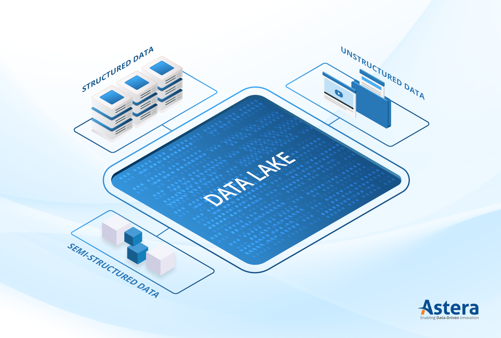
 Handles structured, semi-structured, and unstructured data
 Data Ingestion Layer
 Databases (SQL, NoSQL)
 Storage Layer
 Processing & Analytics Layer
 Security & Governance Layer
 Consumption Layer

 Data Swamp Problem – If not properly managed, a Data Lake can become a “data swamp” (unorganized and unusable).
 Cloud-Based Data Lakes
 Open-Source Data Lake Solutions
 E-Commerce – Customer behavior analysis, recommendation systems.
 Data Lakehouses – A hybrid model combining Data Lake & Data Warehouse capabilities.