Growsoft India

All posts by Madhura babar

Alpha Testing

WHAT IS ALPHA TESTING ?

Alpha Testing


alpha Testing

Alpha testing is an internal form of acceptance testing conducted by an organization’s own employees before releasing a product to external users. It aims to identify bugs and issues within the software to ensure it meets the specified requirements and functions as intended. This testing phase typically involves both black-box and white-box testing techniques and is performed in a controlled environment that simulates real-world usage. 

The alpha testing process generally includes two phases:

  1. Internal Testing by Developers: Developers perform initial tests to identify and fix obvious issues.
  2. Testing by Quality Assurance (QA) Teams: QA teams conduct more thorough testing to uncover additional bugs and assess the software’s overall performance and stability.

By conducting alpha testing, organizations can detect and resolve critical issues early in the development cycle, leading to a more stable and reliable product before it undergoes beta testing with external users

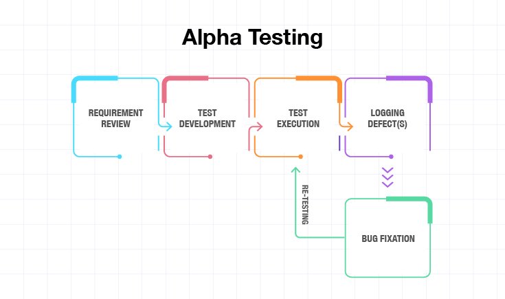
Alpha Testing Process

Alpha testing is a crucial phase in the software development lifecycle, conducted to identify and rectify issues before releasing the product to external users. This internal testing process ensures that the software meets the specified requirements and functions as intended.

The alpha testing process typically involves the following steps:

  1. Requirement Review: Developers and engineers evaluate the software’s specifications and functional requirements, recommending necessary changes to align with project goals.
  2. Test Planning: Based on the requirement review, a comprehensive test plan is developed, outlining the scope, objectives, resources, schedule, and methodologies for testing.
  3. Test Case Design: Detailed test cases are created to cover various scenarios, ensuring that all functionalities are thoroughly examined.
  4. Test Environment Setup: A controlled environment is established to simulate real-world conditions, providing a stable setting for testers to execute test cases.
  5. Test Execution: Testers perform the test cases, documenting any defects, bugs, or performance issues encountered during the process.
  6. Defect Logging and Tracking: Identified issues are logged into a defect-tracking system, detailing their severity, steps to reproduce, and other pertinent information.
  7. Defect Resolution: The development team addresses the reported defects, implementing fixes to resolve the identified issues.
  8. Retesting: After fixes are applied, testers re-execute relevant test cases to confirm that the defects have been successfully resolved and no new issues have arisen.
  9. Regression Testing: To ensure that recent changes haven’t adversely affected existing functionalities, a comprehensive set of tests is run across the application.
  10. Final Evaluation and Reporting: A test summary report is prepared, highlighting the testing outcomes, unresolved issues, and overall product readiness for the next phase, typically beta testing. 

By meticulously following this process, organizations can enhance the quality and reliability of their software products, ensuring a smoother transition to subsequent testing phases and eventual market release.


who perform Alpha Testing ?

Alpha testing is typically conducted by internal teams within an organization. This includes software developers, quality assurance (QA) professionals, and sometimes other employees who are not part of the development team. Developers perform initial tests to identify and fix obvious issues, while QA teams conduct more thorough testing to uncover additional bugs and assess the software’s overall performance and stability. In some cases, non-technical staff may also participate to provide insights into real-world scenarios and user experiences. 


Advantages
Disadvantages
  1. Early Detection of Defects: Identifying and addressing issues during alpha testing helps prevent them from reaching end-users, enhancing the overall quality of the software.
  2. Improved Product Quality: By simulating real-world usage in a controlled environment, alpha testing ensures that the software functions as intended, leading to a more reliable product.
  3. Cost Efficiency: Detecting and fixing bugs early in the development cycle reduces the expenses associated with post-release patches and customer support.
  4. Enhanced Usability: Feedback from internal testers provides insights into the software's usability, allowing developers to make necessary improvements before the beta phase.
  1. Limited Test Coverage: Since alpha testing is conducted internally, it may not cover all possible user scenarios, potentially leaving some issues undiscovered until later stages.
  2. Time-Consuming: Alpha testing can be extensive, requiring significant time to thoroughly evaluate the software, which may delay subsequent testing phases.
  3. Potential Bias: Internal testers, being familiar with the software, might overlook certain issues that external users could encounter, leading to incomplete identification of defects.
  4. Resource Intensive: Conducting comprehensive alpha testing demands considerable resources, including personnel and infrastructure, which might strain project budgets.
Sampling Distribution

SAMPLING DISTRIBUTION

Sampling Distribution
sampling distribution

Sampling Distribution

A sampling distribution is the probability distribution of a statistic (such as the mean, proportion, or standard deviation) obtained from multiple samples drawn from the same population.

In simpler terms, it represents how a sample statistic (like the sample mean) varies when we take multiple samples from the population.

Key Points:

  • It is formed by repeatedly selecting samples from a population and calculating a statistic for each sample.
  • The shape of the sampling distribution depends on the sample size and the population distribution.
  • As the sample size increases, the sampling distribution tends to become more normal due to the Central Limit Theorem (CLT).

Step-by-Step Methods for Sampling Distribution

The process of creating a sampling distribution involves multiple steps, from selecting samples to analyzing their distribution. Here’s a structured step-by-step guide:

Step 1: Define the Population

  • Identify the entire group of individuals or data points you want to study.
  • Example: A university wants to analyze the average height of all its students.

Step 2: Select a Statistic for Analysis

  • Choose a statistic to study, such as: Mean (average), Proportion, Variance
  • Example: If we are studying students’ heights, we focus on the mean height.

Step 3: Take Multiple Random Samples

  • Randomly select multiple samples from the population, ensuring each sample has the same size (n).
  • Example: Take 100 different samples, each containing 50 students.

Step 4: Compute the Sample Statistic

  • Calculate the chosen statistic for each sample.
  • Example: Compute the average height for each sample of 50 students.

Step 5: Create the Sampling Distribution

  • Plot the frequency distribution of the sample statistics (e.g., sample means).
  • This forms the sampling distribution of the mean (if studying averages).

Step 6: Analyze the Shape of the Distribution

  • The shape of the sampling distribution depends on: Sample size (n), Population distribution, Number of samples
  • Key Concept: Central Limit Theorem (CLT)
  • If sample size n is large (n ≥ 30), the sampling distribution will be approximately normal (bell-shaped) even if the population is not normally distributed.

Step 7: Calculate the Mean and Standard Error

  • The mean of the sampling distribution (μₓ̄) is equal to the population mean (μ).
  • The standard deviation of the sampling distribution, called Standard Error (SE) 

Step 8: Apply Statistical Inference

  • Use the sampling distribution to estimate population parameters and make hypothesis tests.
  • Example: If the average sample height is 5.7 feet, we infer the true population mean is around 5.7 feet +- margin of error.
Sampling Distribution

Cluster Sampling

Machine Learning

Cluster Sampling

Cluster sampling is a probability sampling technique where the population is divided into separate groups, called clusters, and a random selection of entire clusters is made. Instead of selecting individuals directly, the researcher selects whole clusters and then collects data from all individuals within the chosen clusters. This method is useful when the population is large and geographically spread out, making it more cost-effective and practical than simple random sampling.
Cluster Sampling


Types of Cluster Sampling

  1. Single-Stage Cluster Sampling: The researcher randomly selects entire clusters and collects data from all individuals within those clusters.
  2. Two-Stage Cluster Sampling: The researcher first randomly selects clusters, and then within those clusters, randomly selects individuals instead of surveying everyone.
  3. Multistage Cluster Sampling: This involves multiple stages of sampling, where clusters are selected at different levels.
  4. Stratified Cluster Sampling: The population is first divided into strata (subgroups), and then clusters are selected within each stratum to ensure better representation.

Examples

  1. Educational Research: A researcher studying students’ academic performance selects 10 schools randomly from a city and surveys all students from those schools instead of selecting students individually from different schools.
  2. Healthcare Studies: A health organization wants to study the eating habits of people in a country. Instead of selecting random individuals, they randomly choose certain cities (clusters) and survey all residents in those cities.
  3. Market Research: A company testing a new product selects 5 shopping malls in different regions and surveys every customer who visits those malls.
  4. Election Polling: To predict election results, a polling agency selects certain districts (clusters) randomly and interviews all voters in those districts instead of selecting individuals across the entire country.
  5. Employee Satisfaction Survey: A company with multiple branches wants to conduct an employee satisfaction survey. Instead of selecting employees randomly from all branches, they randomly pick a few branches and survey all employees in those selected branches.

Methods

Cluster sampling is used when a population is divided into naturally occurring groups (clusters). There are different methods of sample clustering based on how clusters are selected and how data is collected.

1. Single-Stage Cluster Sampling

  • The researcher randomly selects entire clusters from the population.
  • All individuals within the selected clusters are included in the sample.
  • Simple and cost-effective
  • Higher risk of bias if clusters are not representative
  • Example: A researcher selects 5 schools randomly and surveys all students in those schools.

2. Two-Stage Cluster Sampling

  • The researcher first randomly selects clusters from the population.
  • Then, randomly selects individuals within each selected cluster instead of surveying everyone.
  • Reduces sample size while maintaining randomness.
  • More complex than single-stage sampling
  • Example: A researcher selects 5 schools and then randomly picks 50 students from each school instead of surveying all students.

3. Multistage Cluster Sampling

  • Involves multiple levels of sampling where clusters are selected at different stages.
  • Each stage uses random sampling to improve accuracy.
  • More precise and flexible.
  • Requires more resources and time
  • ExampleRandomly select states.

4. Systematic Cluster Sampling

  • Instead of selecting clusters randomly, clusters are selected using a systematic rule (e.g., every 5th cluster).
  • Easy to implement.
  • Can introduce bias if clusters have a pattern
  • Example: A researcher wants to study university students, so they list all universities in a region and select every 3rd university from the list.

5. Stratified Cluster Sampling

  • First, the population is divided into strata (subgroups) based on characteristics like age, gender, or location.
  • Then, clusters are selected within each stratum to ensure better representation.
  • Ensures better representation.
  • More complex and requires prior knowledge of strata
  • Example: If studying workplace satisfaction, companies are first divided into small, medium, and large businesses, and then clusters from each category are selected.

Bagging In Machine Learning

what is Bagging ?

Bagging, an abbreviation for Bootstrap Aggregating, is a powerful ensemble learning technique in machine learning designed to enhance the stability and accuracy of predictive models. By combining the predictions of multiple models trained on different subsets of the data, bagging reduces variance and mitigates the risk of overfitting, leading to more robust and reliable outcomes.

Understanding Bagging

At its core, bagging involves generating multiple versions of a predictor and using these to get an aggregated predictor. The process begins by creating several bootstrap samples from the original dataset. A bootstrap sample is formed by randomly selecting data points from the original dataset with replacement, meaning some data points may appear multiple times in a single sample, while others may be omitted. Each of these samples is then used to train a separate model, often referred to as a base learner. The final prediction is obtained by aggregating the predictions of all base learners, typically through averaging for regression tasks or majority voting for classification tasks.

Bagging in Machine learning

Why Bagging Works ?

Bagging is particularly effective for models that are sensitive to fluctuations in the training data, known as high-variance models. By training multiple models on different subsets of the data and aggregating their predictions, bagging reduces the variance of the final model without increasing the bias. This ensemble approach leads to improved predictive performance and greater robustness.

Bagging, short for Bootstrap Aggregating, is an ensemble learning technique designed to enhance the stability and accuracy of machine learning models. It achieves this by reducing variance and mitigating overfitting, particularly in high-variance models like decision trees.

Bagging, or Bootstrap Aggregating, enhances machine learning models by reducing variance and mitigating overfitting. It involves training multiple models on different subsets of the data and aggregating their predictions. This ensemble approach leads to more stable and accurate predictions. 

Advantages

  1. Variance Reduction: By averaging multiple models, bagging reduces the variance of the prediction, leading to improved performance on unseen data.
  2. Overfitting Mitigation: Combining multiple models helps prevent overfitting, especially in high-variance models like decision trees.
  3. Parallel Training: Each model is trained independently, allowing for parallelization and efficient computation.

Disadvantages

  1. Increased Computational Cost: Training multiple models can be resource-intensive, especially with large datasets or complex models.
  2. Loss of Interpretability: The ensemble of multiple models can be more challenging to interpret compared to a single model

Applications of Bagging

  1. Random Forests: Perhaps the most well-known application of bagging, random forests build an ensemble of decision trees, each trained on a bootstrap sample of the data. Additionally, random forests introduce randomness by selecting a random subset of features for each split in the decision trees, further enhancing diversity among the trees.
  2. Regression and Classification Tasks:Bagging can be applied to various base learners to improve predictive performance in both regression and classification problems.
Bagging in Machine Learning

What is EDA ?

What is EDA ?

What is EDA ?

Exploratory data analysis (EDA) is used by data scientists to analyze and investigate data sets and summarize their main characteristics, often employing data visualization methods.

EDA helps determine how best to manipulate data sources to get the answers you need, making it easier for data scientists to discover patterns, spot anomalies, test a hypothesis, or check assumptions.

EDA is primarily used to see what data can reveal beyond the formal modeling or hypothesis testing task and provides a provides a better understanding of data set variables and the relationships between them. It can also help determine if the statistical techniques you are considering for data analysis are appropriate. Originally developed by American mathematician John Tukey in the 1970s, EDA techniques continue to be a widely used method in the data discovery process today.

Why is EDA Important in Data Science ?

The main purpose of EDA is to help look at data before making any assumptions. It can help identify obvious errors, as well as better understand patterns within the data, detect outliers or anomalous events, find interesting relations among the variables.

Data scientists can use exploratory analysis to ensure the results they produce are valid and applicable to any desired business outcomes and goals. EDA also helps stakeholders by confirming they are asking the right questions. EDA can help answer questions about standard deviations, categorical variables, and confidence intervals. Once EDA is complete and insights are drawn, its features can then be used for more sophisticated data analysis or modeling, including machine learning.


What is EDA ?


EDA Tools

Specific statistical functions and techniques you can perform with EDA tools include : 

  • Clustering and dimension reduction techniques, which help create graphical displays of high-dimensional data containing many variables.

  • Univariate visualization of each field in the raw dataset, with summary statistics.

  • Bivariate visualizations and summary statistics that allow you to assess the relationship between each variable in the dataset and the target variable you’re looking at.

  • Multivariate visualizations, for mapping and understanding interactions between different fields in the data.

  • K-means clustering, which is a clustering method in unsupervised learning where data points are assigned into K groups, i.e. the number of clusters, based on the distance from each group’s centroid. The data points closest to a particular centroid will be clustered under the same category. K-means clustering is commonly used in market segmentation, pattern recognition, and image compression.

  • Predictive models, such as linear regression, use statistics and data to predict outcomes. 


EDA Techniques

Some of the common techniques and methods used in Exploratory Data Analysis include the following:

Data Visualization

Data visualization involves generating visual representations of the data using graphs, charts, and other graphical techniques. Data visualization enables a quick and easy understanding of patterns and relationships within data. Visualization techniques include scatter plots, histograms, heatmaps and box plots

Correlation Analysis

Using correlation analysis, one can analyze the relationships between pairs of variables to identify any correlations or dependencies between them. Correlation analysis helps in feature selection and in building predictive models. Common correlation techniques include Pearson’s correlation coefficient, Spearman’s rank correlation coefficient and Kendall’s tau correlation coefficient.

Dimensionality Reduction

In dimensionality reduction, techniques like principal component analysis (PCA) and linear discriminant analysis (LDA) are used to decrease the number of variables in the data while keeping as many details as possible.

Descriptive Statistics

It involves calculating summary statistics such as mean, median, mode, standard deviation and variance to gain insights into the distribution of data. The mean is the average value of the data set and provides an idea of the central tendency of the data. The median is the mid-value in a sorted list of values and provides another measure of central tendency. The mode is the most common value in the data set.

Clustering

Clustering techniques such as K-means clustering, hierarchical clustering, and DBSCAN clustering help identify patterns and relationships within a dataset by grouping similar data points together based on their characteristics.

Outlier Detection

Outliers are data points that vary or deviate significantly from the rest of the data and can have a crucial impact on the accuracy of models. Identifying and removing outliers from data using methods like Z-score, interquartile range (IQR) and box plots method can help improve the data quality and the models’ accuracy.


Types Of EDA

Univariate non-graphical

This is simplest form of data analysis, where the data being analyzed consists of just one variable. Since it’s a single variable, it doesn’t deal with causes or relationships. The main purpose of univariate analysis is to describe the data and find patterns that exist within it.

Univariate graphical

Non-graphical methods don’t provide a full picture of the data. Graphical methods are therefore required. Common types of univariate graphics include:

  • Stem-and-leaf plots, which show all data values and the shape of the distribution.
  • Histograms, a bar plot in which each bar represents the frequency (count) or proportion (count/total count) of cases for a range of values.
  • Box plots, which graphically depict the five-number summary of minimum, first quartile, median, third quartile, and maximum.
Multivariate non-graphical

Multivariate data arises from more than one variable. Multivariate non-graphical EDA techniques generally show the relationship between two or more variables of the data through cross-tabulation or statistics.

Multivariate graphical

Multivariate data uses graphics to display relationships between two or more sets of data. The most used graphic is a grouped bar plot or bar chart with each group representing one level of one of the variables and each bar within a group representing the levels of the other variable.

Other common types of multivariate graphics include:

  • Scatter plot, which is used to plot data points on a horizontal and a vertical axis to show how much one variable is affected by another.
  • Multivariate chart, which is a graphical representation of the relationships between factors and a response.
  • Run chart, which is a line graph of data plotted over time.
  • Bubble chart, which is a data visualization that displays multiple circles (bubbles) in a two-dimensional plot.
  • Heat map, which is a graphical representation of data where values are depicted by color.

Exploratory Data Analysis Languages

Some of the most common data science programming languages used to create an EDA include:

   Python :
  • An interpreted, object-oriented programming language with dynamic semantics. Its high-level, built-in data structures, combined with dynamic typing and dynamic binding, make it very attractive for rapid application development, as well as for use as a scripting or glue language to connect existing components together. Python and EDA can be used together to identify missing values in a data set, which is important so you can decide how to handle missing values for machine learning.

      R :

  • An open-source programming language and free software environment for statistical computing and graphics supported by the R Foundation for Statistical Computing. The R language is widely used among statisticians in data science in developing statistical observations and data analysis.